High-Demand Utilities in Virginia: Statistical Learning Project CODE

Exploratory Data Analysis

The following code is used in the Exploratory Data Analysis section.

library(dplyr)
library(tidyr)
library(ggplot2)
library(readr)
library(stringr)
library(reshape2)

theme_set(theme_minimal())

elec_2023 <- read_csv("data/power/electricity_2023.csv")
elec_all  <- read_csv("data/power/electricity_2015_to_2024.csv")

# glimpse(elec_2023)
# glimpse(elec_all)

############################################################
## Data Cleaning & Feature Engineering
############################################################

# Utility to build features and clean data 
# - is_VA classifies obs if Utility.State == "VA"
# - Filter out certain important fields that are zero
# - Feature engineer 
featurize_utilities_raw <- function(df) {
  df %>%
    mutate(
      is_VA = if_else(Utility.State == "VA", 1L, 0L)
    ) %>%
    filter(
      Retail.Total.Customers > 0,
      Retail.Total.Sales > 0,
      Uses.Total > 0
    ) %>%
    mutate(
      Commercial_Ratio = Retail.Commercial.Sales / Retail.Total.Sales,
      Residential_Ratio = Retail.Residential.Sales / Retail.Total.Sales,
      Industrial_Ratio = Retail.Industrial.Sales / Retail.Total.Sales,
      SalesPerCustomer = Retail.Total.Sales / Retail.Total.Customers,
      Commercial_SPC = if_else(Retail.Commercial.Customers > 0,
                                    Retail.Commercial.Sales / Retail.Commercial.Customers,
                                    NA_real_),
      Residential_SPC = if_else(Retail.Residential.Customers > 0,
                                    Retail.Residential.Sales / Retail.Residential.Customers,
                                    NA_real_),
      Losses_Ratio = Uses.Losses / Uses.Total,
      log_Total_Sales = log(Retail.Total.Sales),
      log_Total_Customers = log(Retail.Total.Customers)
    )
}
 
elec_2023_fe <- featurize_utilities_raw(elec_2023)
elec_all_fe  <- featurize_utilities_raw(elec_all)

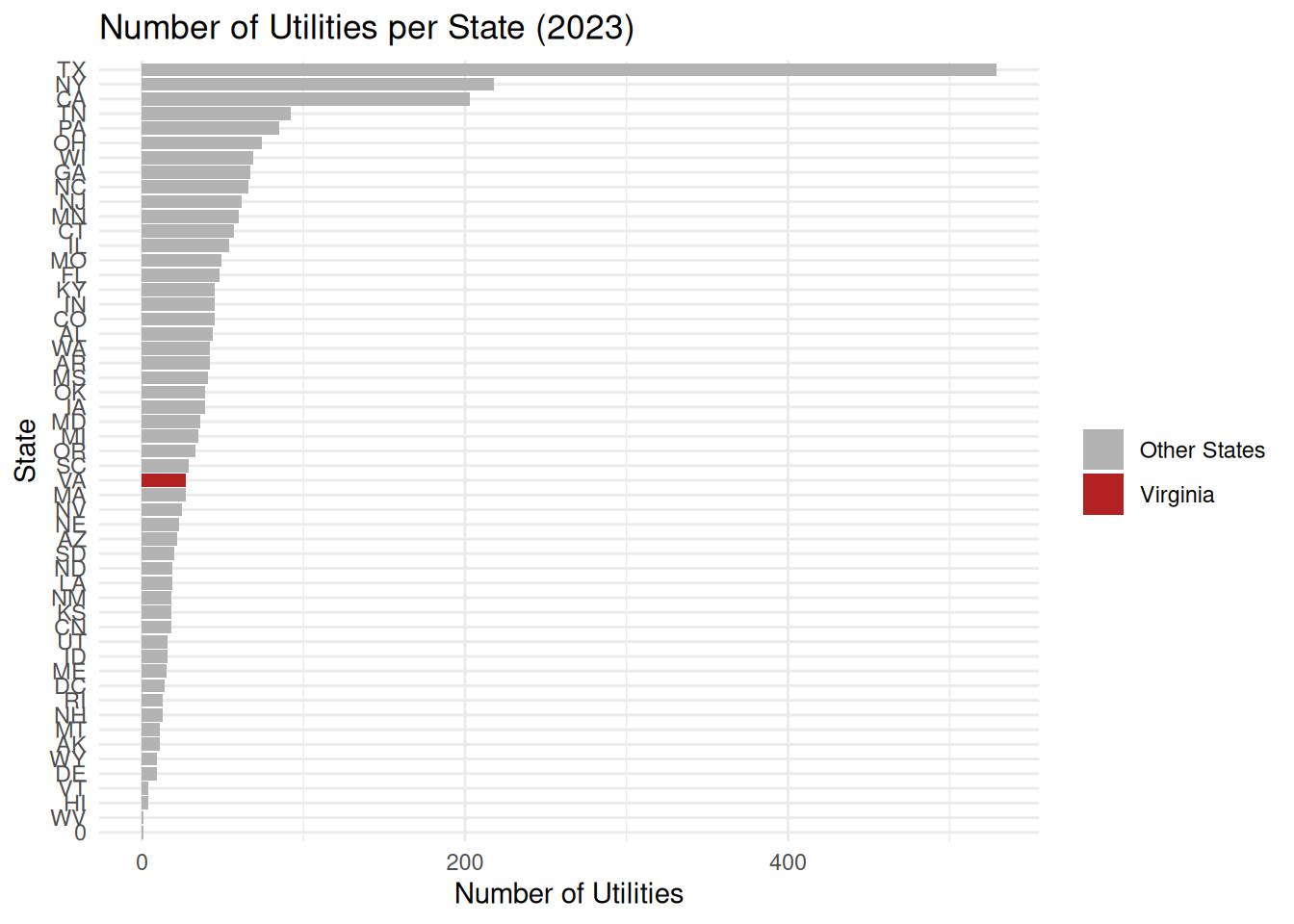
state_counts_2023 <- elec_2023_fe %>%
  count(Utility.State, sort = TRUE) %>%
  mutate(
    Highlight = if_else(Utility.State == "VA", "Virginia", "Other States")
  )

ggplot(state_counts_2023,
       aes(x = reorder(Utility.State, n), y = n, fill = Highlight)) +
  geom_col() +
  coord_flip() +
  scale_fill_manual(values = c("Virginia" = "firebrick", "Other States" = "grey70")) +
  labs(
    title = "Number of Utilities per State (2023)",
    x = "State",
    y = "Number of Utilities",
    fill = ""
  )

Figure 1: Number of utilities per state in 2023, with Virginia highlighted.

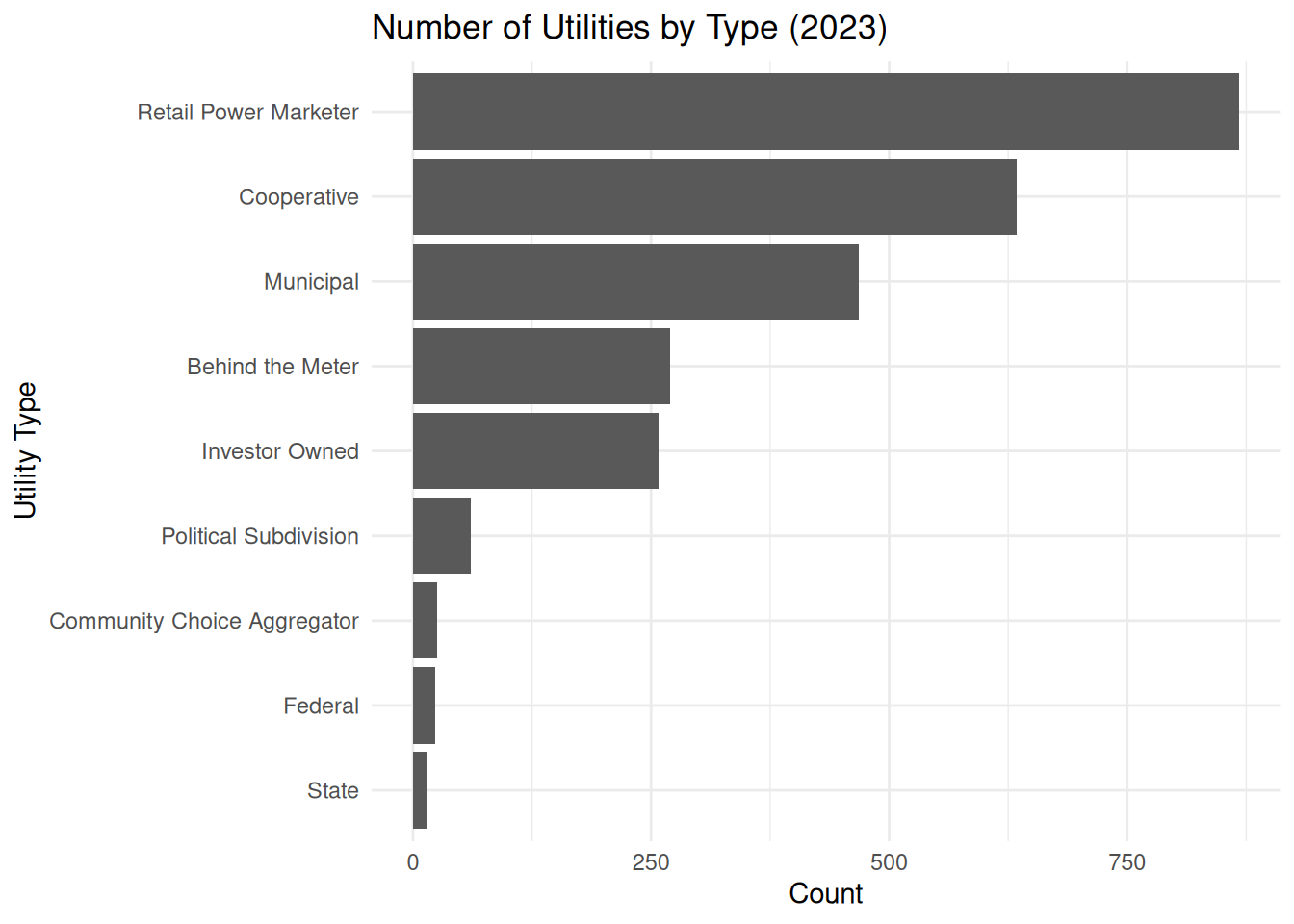
type_counts_2023 <- elec_2023_fe %>%
  count(Utility.Type, sort = TRUE)

ggplot(type_counts_2023,
       aes(x = reorder(Utility.Type, n), y = n)) +
  geom_col() +
  coord_flip() +
  labs(
    title = "Number of Utilities by Type (2023)",
    x = "Utility Type",
    y = "Count"
  )

Figure 2: Number of utilities by type in 2023.

############################################################
## Distribution Plots for Key Numeric Variables (2023)
############################################################

candidate_numeric_cols <- c(
  "Demand.Summer.Peak",
  "Demand.Winter.Peak",
  "Sources.Generation",
  "Sources.Purchased",
  "Uses.Total",
  "Retail.Residential.Sales",
  "Retail.Commercial.Sales",
  "Retail.Industrial.Sales",
  "Retail.Total.Sales",
  "Retail.Total.Customers"
)

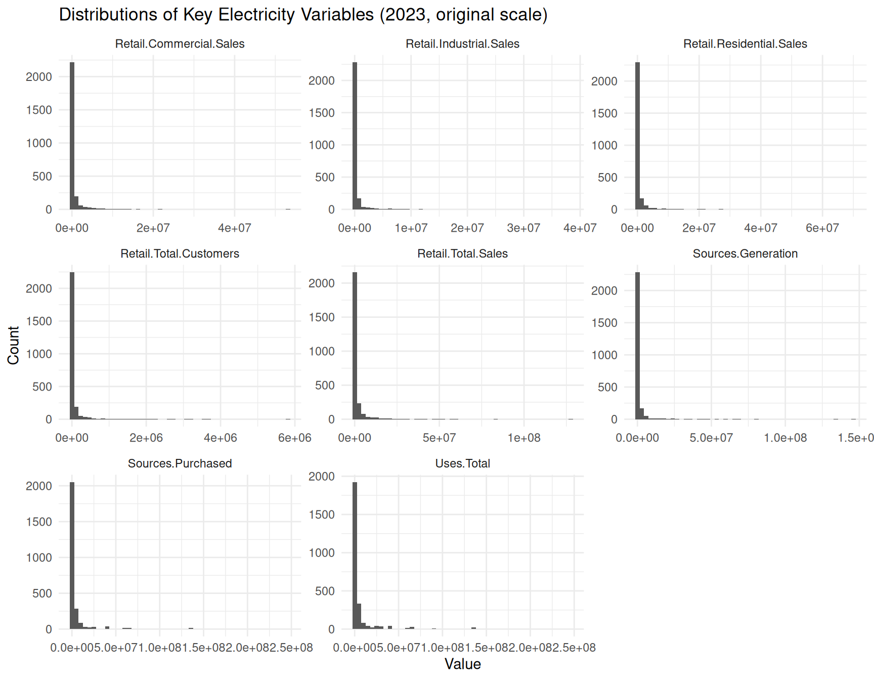
num_vars_2023 <- elec_2023_fe %>%
  select(any_of(candidate_numeric_cols))

num_long_2023 <- num_vars_2023 %>%
  tidyr::pivot_longer(
    everything(),
    names_to = "variable",
    values_to = "value"
  )

ggplot(num_long_2023, aes(x = value)) +
  geom_histogram(bins = 50) +
  facet_wrap(~ variable, scales = "free") +
  labs(
    title = "Distributions of Key Electricity Variables (2023, original scale)",
    x = "Value",
    y = "Count"
  )

Figure 3: Distributions of key electricity variables in 2023 (original scale).

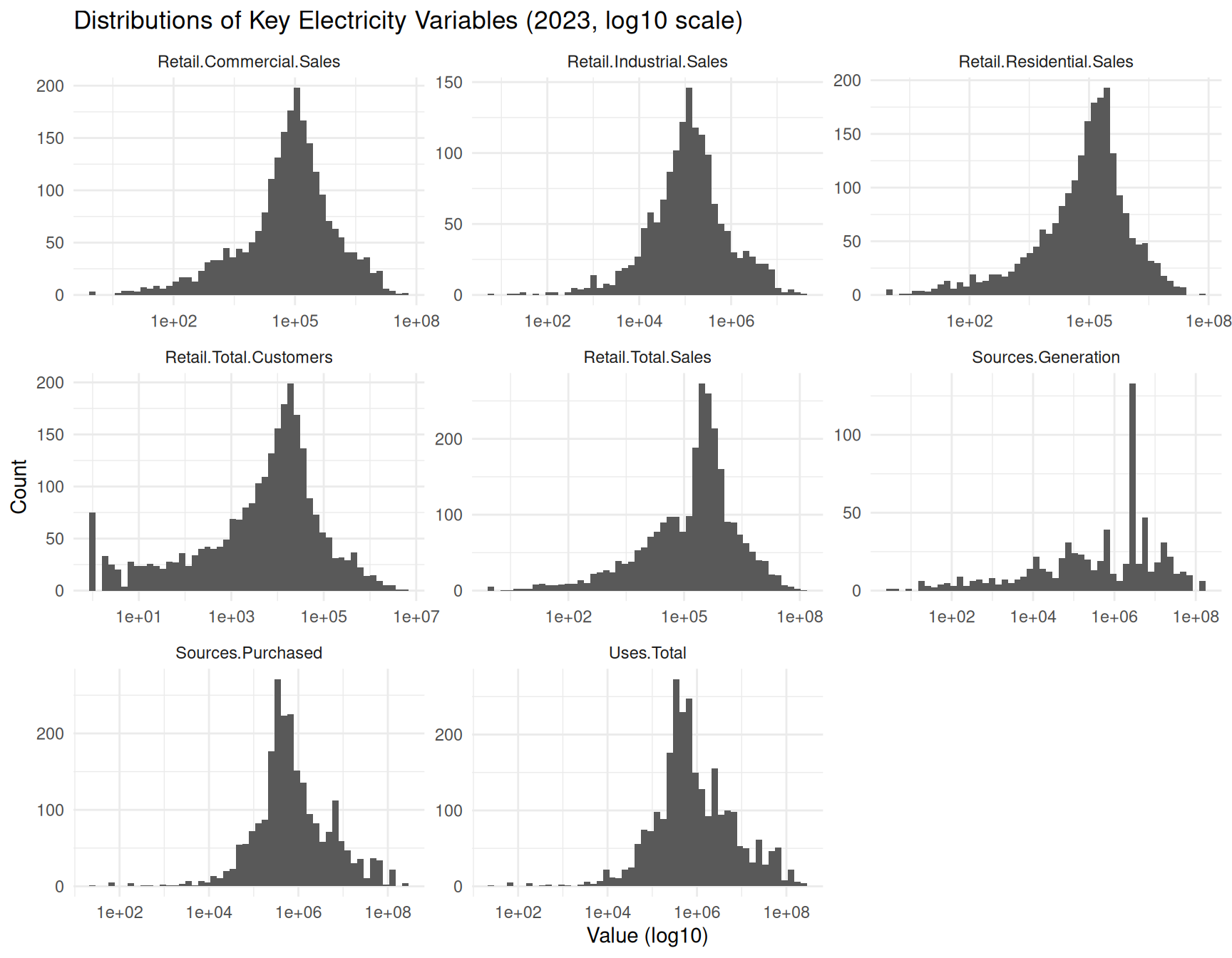
ggplot(num_long_2023, aes(x = value)) +
  geom_histogram(bins = 50) +
  facet_wrap(~ variable, scales = "free") +
  scale_x_log10() +
  labs(
    title = "Distributions of Key Electricity Variables (2023, log10 scale)",
    x = "Value (log10)",
    y = "Count"
  )

Figure 4: Distributions of key electricity variables in 2023 (log10 scale).

############################################################
## Sector Mix & Ratios (2023, including Virginia vs Others)
############################################################

ratio_long_2023 <- elec_2023_fe %>%
  select(
    Utility.State, is_VA,
    Commercial_Ratio, Residential_Ratio,
    Industrial_Ratio, Losses_Ratio
  ) %>%
  tidyr::pivot_longer(
    cols = c(Commercial_Ratio, Residential_Ratio, Industrial_Ratio, Losses_Ratio),
    names_to = "ratio_type",
    values_to = "value"
  )

ggplot(ratio_long_2023,
       aes(x = value)) +
  geom_histogram(bins = 50) +
  facet_wrap(~ ratio_type, scales = "free") +
  labs(
    title = "Distribution of Sector Ratios (2023)",
    x = "Ratio",
    y = "Count"
  )

Figure 5: Distribution of key electricity sector ratios across all U.S. utilities in 2023.

ratio_long_2023_va <- ratio_long_2023 %>%
  mutate(
    Region = if_else(is_VA == 1L, "Virginia", "Other States")
  )

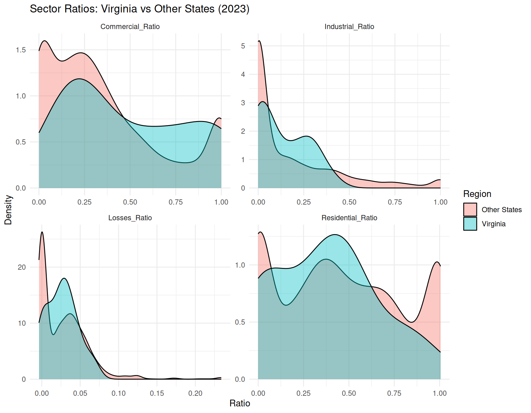
ggplot(ratio_long_2023_va,
       aes(x = value, fill = Region)) +
  geom_density(alpha = 0.4) +
  facet_wrap(~ ratio_type, scales = "free") +
  labs(
    title = "Sector Ratios: Virginia vs Other States (2023)",
    x = "Ratio",
    y = "Density",
    fill = "Region"
  )

Figure 6: Comparison of sector ratios between Virginia utilities and all other U.S. utilities in 2023.

spc_long_2023 <- elec_2023_fe %>%
  dplyr::select(
    is_VA,
    SalesPerCustomer,
    Commercial_SPC,
    Residential_SPC
  ) %>%
  tidyr::pivot_longer(
    cols = c(SalesPerCustomer, Commercial_SPC, Residential_SPC),
    names_to = "metric",
    values_to = "value"
  ) %>%
  dplyr::mutate(
    Region = if_else(is_VA == 1L, "Virginia", "Other States")
  )

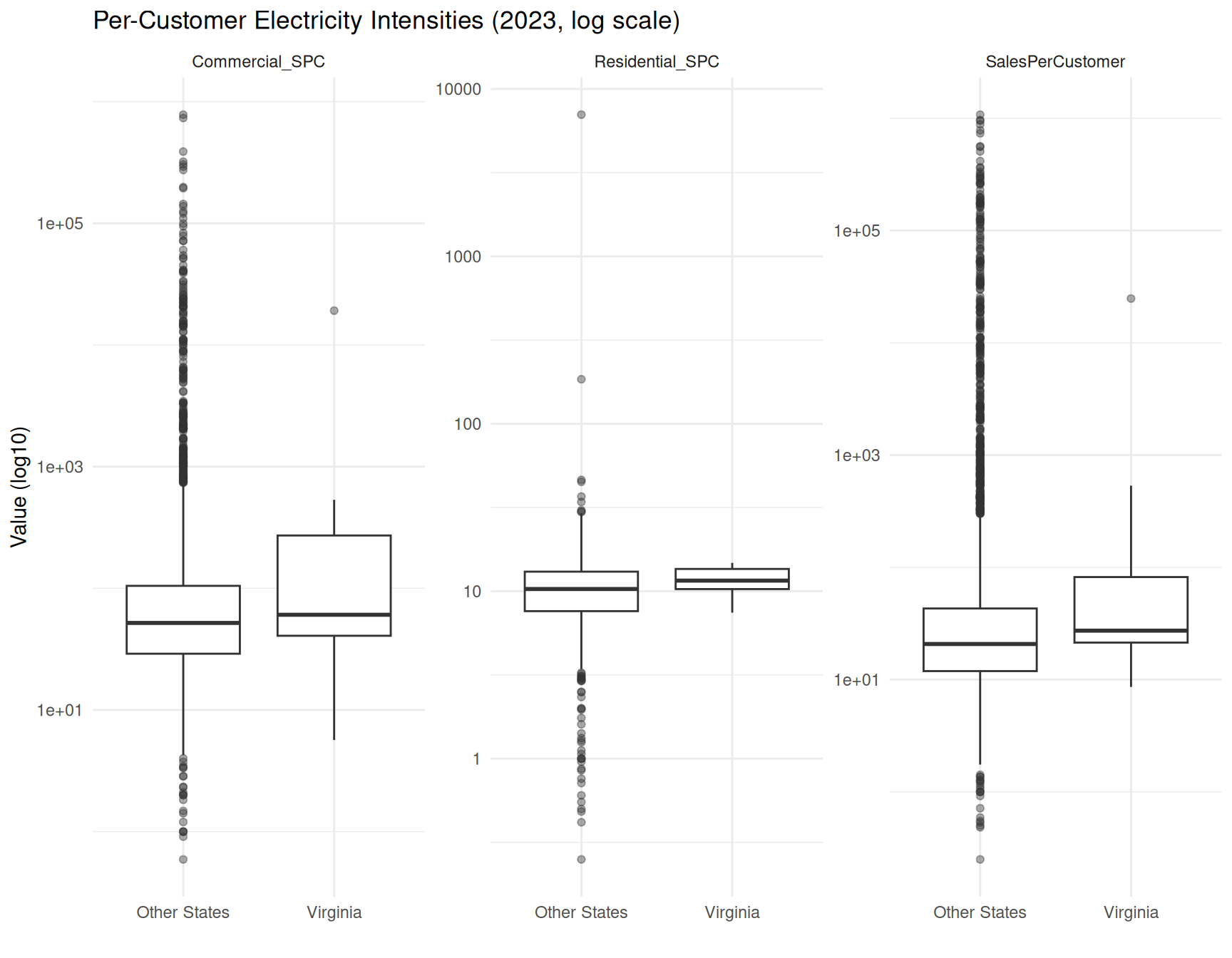
ggplot(spc_long_2023,
       aes(x = Region, y = value)) +
  geom_boxplot(outlier.alpha = 0.4) +
  facet_wrap(~ metric, scales = "free_y") +
  scale_y_log10() +
  labs(
    title = "Per-Customer Electricity Intensities (2023, log scale)",
    x = "",
    y = "Value (log10)"
  )

Figure 7: Comparison of per-customer electricity intensity measures for Virginia utilities versus all other U.S. utilities (2023). Values shown on a log scale.

ggplot(elec_2023_fe,
       aes(x = Retail.Total.Customers,
           y = Retail.Total.Sales,
           color = factor(is_VA))) +
  geom_point(alpha = 0.6) +
  scale_x_log10() +
  scale_y_log10() +
  labs(
    title = "Total Sales vs Total Customers (2023)",
    x = "Total Customers (log10)",
    y = "Total Sales (log10)",
    color = "Virginia (1 = VA)"
  ) +
  scale_color_manual(values = c("0" = "gray60", "1" = "red"))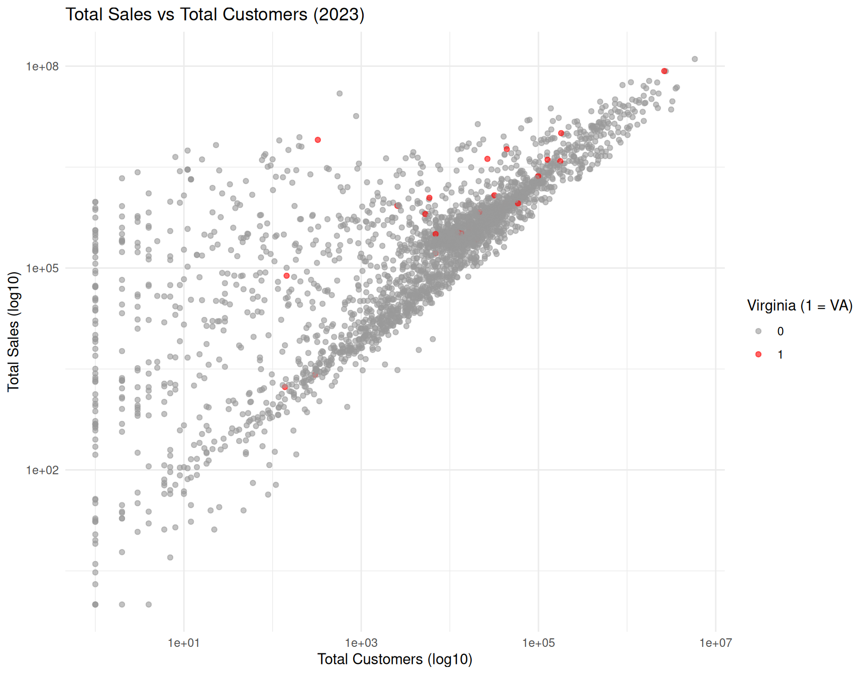

Figure 8: Relationship between total customers and total electricity sales (log–log scale) for U.S. utilities in 2023, highlighting Virginia utilities.

ggplot(elec_2023_fe,
       aes(x = Commercial_Ratio,
           y = Commercial_SPC,
           color = factor(is_VA))) +
  geom_point(alpha = 0.6) +
  scale_y_log10() +
  labs(
    title = "Commercial Ratio vs Commercial Sales per Customer (2023)",
    x = "Commercial Ratio",
    y = "Commercial Sales per Commercial Customer (log10)",
    color = "Virginia (1 = VA)"
  ) +
  scale_color_manual(values = c("0" = "gray60", "1" = "red"))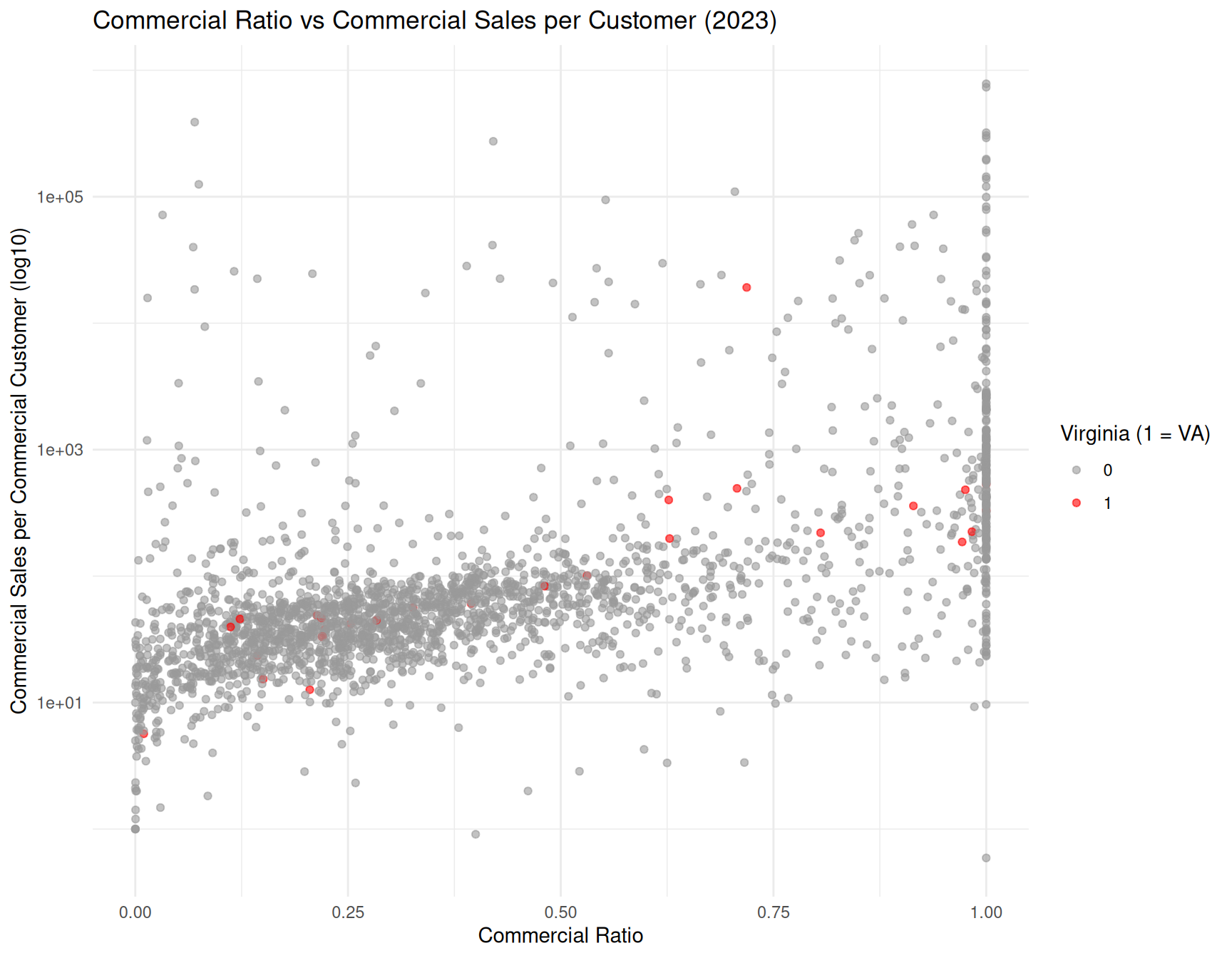

Figure 9: Commercial sector structure versus commercial sales per customer (log scale) for U.S. utilities in 2023, with Virginia utilities highlighted.

va_vs_us_year <- elec_all_fe %>%
  mutate(Region = if_else(Utility.State == "VA", "Virginia", "Other States")) %>%
  group_by(Year, Region) %>%
  summarise(
    total_sales          = sum(Retail.Total.Sales, na.rm = TRUE),
    total_customers      = sum(Retail.Total.Customers, na.rm = TRUE),
    avg_SalesPerCustomer = mean(SalesPerCustomer, na.rm = TRUE),
    avg_Commercial_Ratio = mean(Commercial_Ratio, na.rm = TRUE),
    .groups = "drop"
  )

ggplot(va_vs_us_year,
       aes(x = Year, y = avg_SalesPerCustomer, color = Region)) +
  geom_line(size = 1) +
  labs(
    title = "Average Sales per Customer: Virginia vs Other States (2015–2024)",
    x = "Year",
    y = "Average Sales per Customer",
    color = "Region"
  ) +
  scale_color_manual(values = c("Virginia" = "red", "Other States" = "gray40"))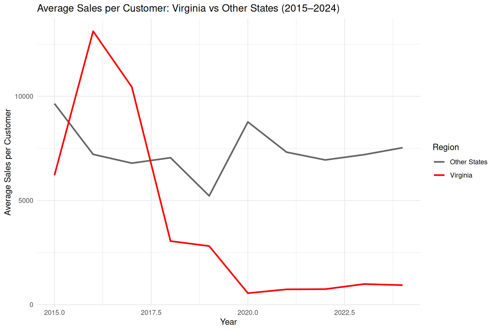

Figure 10: Average electricity sales per customer over time (2015–2024), comparing Virginia to all other U.S. states.

ggplot(va_vs_us_year,
       aes(x = Year, y = avg_Commercial_Ratio, color = Region)) +
  geom_line(size = 1) +
  labs(
    title = "Average Commercial Ratio: Virginia vs Other States (2015–2024)",
    x = "Year",
    y = "Average Commercial Ratio",
    color = "Region"
  ) +
  scale_color_manual(values = c("Virginia" = "red", "Other States" = "gray40"))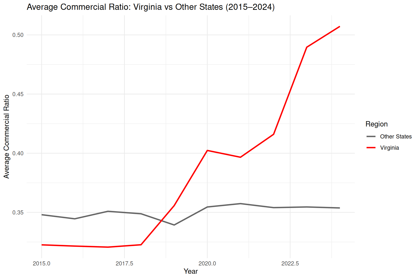

Figure 11: Average commercial electricity sales ratio over time (2015–2024), comparing Virginia to all other U.S. states.

Building Classifiers

The following code is used in the Building Classifiers section.

library(glmnet) # ridge logistic
library(rpart) # classification tree
library(rpart.plot) # tree plot
library(randomForest) # random forest
library(class) # KNN
library(knitr)
library(kableExtra)

set.seed(123)

power_combined <- read.csv("data/power/electricity_2015_to_2024.csv")

featurize_utilities <- function(df_raw) {
  df_raw %>%
    filter(
      Retail.Total.Customers > 0,
      Retail.Total.Sales > 0,
      Retail.Commercial.Customers > 0,
      Retail.Commercial.Sales > 0,
      Uses.Total > 0
    ) %>%
    # Drop retail power marketers to avoid distorting commercial ratio
    filter(Utility.Type != "Retail Power Marketer") %>%
    mutate(
      Commercial_Ratio = Retail.Commercial.Sales / Retail.Total.Sales,
      SalesPerCustomer = Retail.Total.Sales / Retail.Total.Customers,
      Commercial_SPC = Retail.Commercial.Sales / Retail.Commercial.Customers,
      Losses_Ratio = Uses.Losses / Uses.Total,
      log_Total_Sales = log(Retail.Total.Sales),
      log_Total_Customers = log(Retail.Total.Customers),
      is_VA = if_else(Utility.State == "VA", 1L, 0L)
    )
}

train_year <- 2023

df_year <- power_combined %>%
  filter(Year == train_year) %>%
  featurize_utilities()

# Create z-scores and composite IntensityScore
df_year <- df_year %>%
  mutate(
    z_Commercial_Ratio = as.numeric(scale(Commercial_Ratio)),
    z_SalesPerCustomer = as.numeric(scale(SalesPerCustomer)),
    z_Commercial_SPC = as.numeric(scale(Commercial_SPC))
  ) %>%
  mutate(
    IntensityScore = z_Commercial_Ratio +
                     z_SalesPerCustomer +
                     z_Commercial_SPC
  )

# High-demand = top 10% of intensity
cutoff <- quantile(df_year$IntensityScore, 0.90, na.rm = TRUE)

df_year <- df_year %>%
  mutate(
    HighDemand_intensity = if_else(IntensityScore >= cutoff, 1L, 0L)
  )

df_year %>%
  count(HighDemand_intensity) %>%
  ggplot(aes(x = factor(HighDemand_intensity),
             y = n,
             fill = factor(HighDemand_intensity))) +
  geom_col() +
  geom_text(aes(label = n),
            vjust = -0.4,
            size = 5,
            fontface = "bold") +
  scale_fill_manual(values = c("#4C78A8", "#F58518"),
                    name = "High Demand",
                    labels = c("0 = Normal Demand", "1 = High Demand")) +
  labs(
    title = "Counts of High-Demand vs Normal-Demand Utilities (2023)",
    x = "High Demand Indicator",
    y = "Count"
  ) +
  theme_minimal(base_size = 14)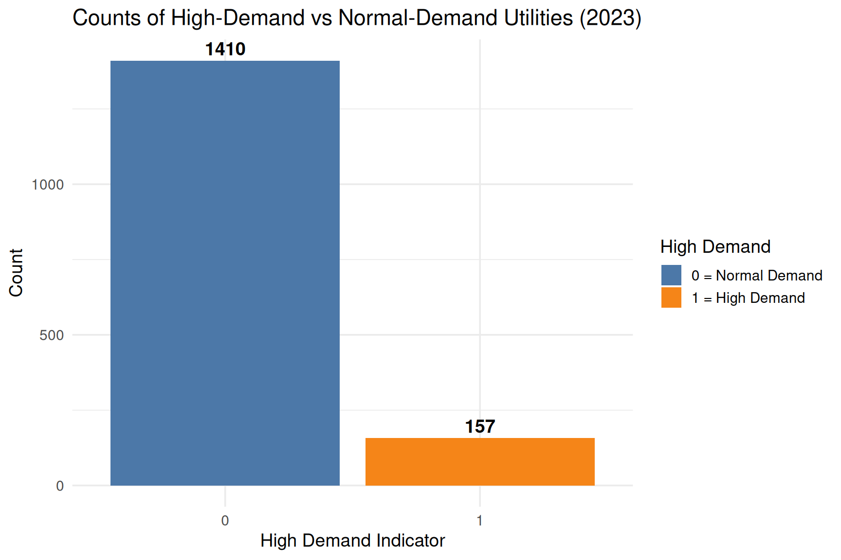

Figure 12: Distribution of high demand utilities for (2023)

eda_vars <- c(
  "Commercial_Ratio",
  "SalesPerCustomer",
  "Commercial_SPC",
  "Losses_Ratio",
  "log_Total_Customers"
)

df_long <- df_year %>%
  select(all_of(eda_vars), HighDemand_intensity) %>%
  pivot_longer(cols = all_of(eda_vars),
               names_to = "variable",
               values_to = "value")

# Histograms (original scale)
ggplot(df_long, aes(x = value)) +
  geom_histogram(bins = 50) +
  facet_wrap(~ variable, scales = "free") +
  theme_minimal() +
  labs(title = "Distributions of Predictors (original scale)")

Figure 13: Distributions of Predictors (original scale)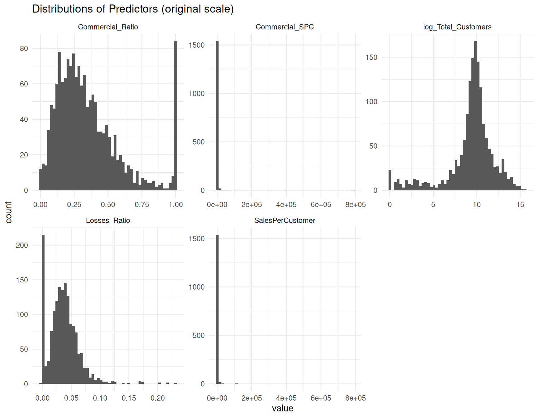

# Histograms (log scale) to show skew
ggplot(df_long, aes(x = value)) +
  geom_histogram(bins = 50) +
  facet_wrap(~ variable, scales = "free") +
  scale_x_log10() +
  theme_minimal() +
  labs(title = "Distributions of Predictors (log10 scale)")

Figure 14: Distributions of Predictors (log10 scale)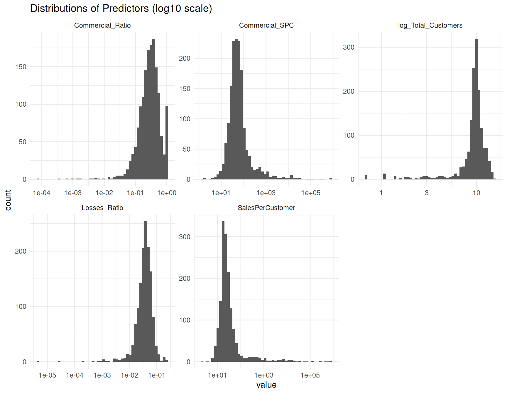

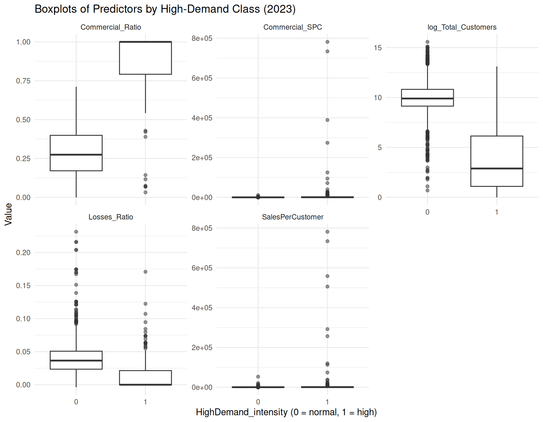
# Boxplots by high-demand class
ggplot(df_long,
       aes(x = factor(HighDemand_intensity), y = value)) +
  geom_boxplot(outlier.alpha = 0.5) +
  facet_wrap(~ variable, scales = "free_y") +
  theme_minimal() +
  labs(
    x = "HighDemand_intensity (0 = normal, 1 = high)",
    y = "Value",
    title = "Boxplots of Predictors by High-Demand Class (2023)"
  )

Figure 15: Boxplots of Predictors by High-Demand Class (2023)

Logistic Regression

The following code is used in the Logistic Regression section.

############################################################
## Train/Test Split (for 2023 models)
############################################################

n <- nrow(df_year)
set.seed(123)
train_idx <- sample(seq_len(n), size = 0.8 * n)

train <- df_year[train_idx, ]
test <- df_year[-train_idx, ]

train$Utility.Type <- factor(train$Utility.Type)
test$Utility.Type <- factor(test$Utility.Type)

############################################################
## Raw Logistic Regression Model
############################################################

model_raw <- glm(
  HighDemand_intensity ~ Commercial_Ratio + SalesPerCustomer +
    Commercial_SPC + Losses_Ratio + log_Total_Customers +
    is_VA + Utility.Type,
  data = train,
  family = binomial
)

# summary(model_raw)  # shows separation / huge coefficients

test$pred_prob_raw <- predict(model_raw, newdata = test, type = "response")
test$pred_class_raw <- ifelse(test$pred_prob_raw >= 0.5, 1L, 0L)

confusion_raw <- table(
  Predicted = test$pred_class_raw,
  Actual    = test$HighDemand_intensity
)

# Basic, theme-friendly table
kable(
  confusion_raw,
  caption = "Confusion Matrix",
  align = "c"
)
# Accuracy as a small table under it
accuracy_raw <- mean(test$pred_class_raw == test$HighDemand_intensity)

kable(
  data.frame(`Classification Accuracy` = round(accuracy_raw, 4)),
  align = "c"
)

Table 1: Confusion Matrix for Unpenalized Logistic Regression Model (Test Set)

Confusion Matrix

	0	1
0	274	6
1	1	33

Classification.Accuracy
0.9777

############################################################
# Standardized Logistic Model
############################################################

scale_vars <- c(
  "Commercial_Ratio",
  "SalesPerCustomer",
  "Commercial_SPC",
  "Losses_Ratio",
  "log_Total_Customers"
)

df_year_std <- df_year %>%
  mutate(across(
    all_of(scale_vars),
    ~ as.numeric(scale(.x)),
    .names = "s_{.col}"
  ))

train_std <- df_year_std[train_idx, ]
test_std  <- df_year_std[-train_idx, ]

train_std$Utility.Type <- factor(train_std$Utility.Type)
test_std$Utility.Type  <- factor(test_std$Utility.Type)

model_std <- glm(
  HighDemand_intensity ~ s_Commercial_Ratio + s_SalesPerCustomer +
    s_Commercial_SPC + s_Losses_Ratio + s_log_Total_Customers +
    is_VA + Utility.Type,
  data = train_std,
  family = binomial
)

# summary(model_std)

test_std$pred_prob_std <- predict(model_std, newdata = test_std, type = "response")
test_std$pred_class_std <- ifelse(test_std$pred_prob_std >= 0.5, 1L, 0L)

confusion_std <- table(
  Predicted = test_std$pred_class_std,
  Actual    = test_std$HighDemand_intensity
)

kable(
  confusion_std,
  caption = "Confusion Matrix (Standardized Logistic Model)",
  align = "c"
)
# Classification accuracy
accuracy_std <- mean(test_std$pred_class_std == test_std$HighDemand_intensity)

kable(
  data.frame(`Classification Accuracy` = round(accuracy_std, 4)),
  align = "c"
)

Table 2: Confusion Matrix for Standardized Logistic Regression Model (Test Set)

Confusion Matrix (Standardized Logistic Model)

	0	1
0	274	6
1	1	33

Classification.Accuracy
0.9777

############################################################
# Ridge Logistic Regression
############################################################

formula_all <- HighDemand_intensity ~ Commercial_Ratio + SalesPerCustomer +
  Commercial_SPC + Losses_Ratio + log_Total_Customers +
  is_VA + Utility.Type

x_train <- model.matrix(formula_all, data = train)[, -1]
y_train <- train$HighDemand_intensity

ridge_x_cols <- colnames(x_train)

x_test  <- model.matrix(formula_all, data = test)[, -1]
y_test  <- test$HighDemand_intensity

ridge_cv <- cv.glmnet(
  x_train,
  y_train,
  family = "binomial",
  alpha = 0
)

# plot(ridge_cv, main = "Ridge Logistic: CV Error vs Lambda") -->
# best_lambda <- ridge_cv$lambda.min -->
# best_lambda -->

pred_prob_ridge_test <- predict(ridge_cv, newx = x_test,
                                s = "lambda.min", type = "response")
pred_class_ridge_test <- ifelse(pred_prob_ridge_test >= 0.5, 1L, 0L)

# Confusion matrix
confusion_ridge <- table(
  Predicted = pred_class_ridge_test,
  Actual    = y_test
)

kable(
  confusion_ridge,
  caption = "Confusion Matrix (Ridge Logistic Model)",
  align = "c"
)
# Accuracy table
accuracy_ridge <- mean(pred_class_ridge_test == y_test)

kable(
  data.frame(`Classification Accuracy` = round(accuracy_ridge, 4)),
  align = "c"
)

Table 3: Confusion Matrix for Ridge Logistic Regression Model (Test Set)

Confusion Matrix (Ridge Logistic Model)

	0	1
0	275	17
1	0	22

Classification.Accuracy
0.9459

model_comparison <- data.frame(
  Model = c(
    "Raw Logistic Regression",
    "Standardized Logistic Regression",
    "Ridge Logistic Regression"
  ),
  `Training Issues` = c(
    "Severe separation; coefficients explode",
    "Still unstable; separation persists",
    "Stable; L2 penalty prevents divergence"
  ),
  `Interpretability` = c(
    "Poor (coefficients meaningless)",
    "Poor (scaled version of same issue)",
    "Moderate (penalized, but stable)"
  ),
  `AIC` = c(
    604.7,
    604.7,
    NA   # glmnet does not compute AIC
  ),
  `Test Accuracy` = c(
    round(accuracy_raw, 4),
    round(accuracy_std, 4),
    round(accuracy_ridge, 4)
  ),
  `Key Notes` = c(
    "Not reliable for inference; unstable estimates",
    "Standardization alone did not fix the problem",
    "Best predictive model; generalizes well"
  )
)

kable(model_comparison, align = "c")

Table 4: Comparison of Logistic Regression Models for High-Demand Classification

Model	Training.Issues	Interpretability	AIC	Test.Accuracy	Key.Notes
Raw Logistic Regression	Severe separation; coefficients explode	Poor (coefficients meaningless)	604.7	0.9777	Not reliable for inference; unstable estimates
Standardized Logistic Regression	Still unstable; separation persists	Poor (scaled version of same issue)	604.7	0.9777	Standardization alone did not fix the problem
Ridge Logistic Regression	Stable; L2 penalty prevents divergence	Moderate (penalized, but stable)	NA	0.9459	Best predictive model; generalizes well

Tree Classifier

The following code is used in the Tree Classifier section.

############################################################
## Classification Tree 
############################################################

#Tree Model
tree_model <- rpart(
  HighDemand_intensity ~ Commercial_Ratio + SalesPerCustomer +
    Commercial_SPC + Losses_Ratio + log_Total_Customers +
    is_VA + Utility.Type,
  data = train,
  method = "class"
)

#Tree Visualization
rpart.plot(tree_model, main = "Classification Tree for High-Demand Utilities")
print(tree_model)

n= 1253 

node), split, n, loss, yval, (yprob)
      * denotes terminal node

1) root 1253 118 0 (0.905826018 0.094173982)  
  2) Commercial_Ratio< 0.7096691 1144   9 0 (0.992132867 0.007867133)  
    4) Commercial_SPC< 12663.81 1135   0 0 (1.000000000 0.000000000) *
    5) Commercial_SPC>=12663.81 9   0 1 (0.000000000 1.000000000) *
  3) Commercial_Ratio>=0.7096691 109   0 1 (0.000000000 1.000000000) *

#Tree Predictions
tree_pred <- predict(tree_model, newdata = test, type = "class")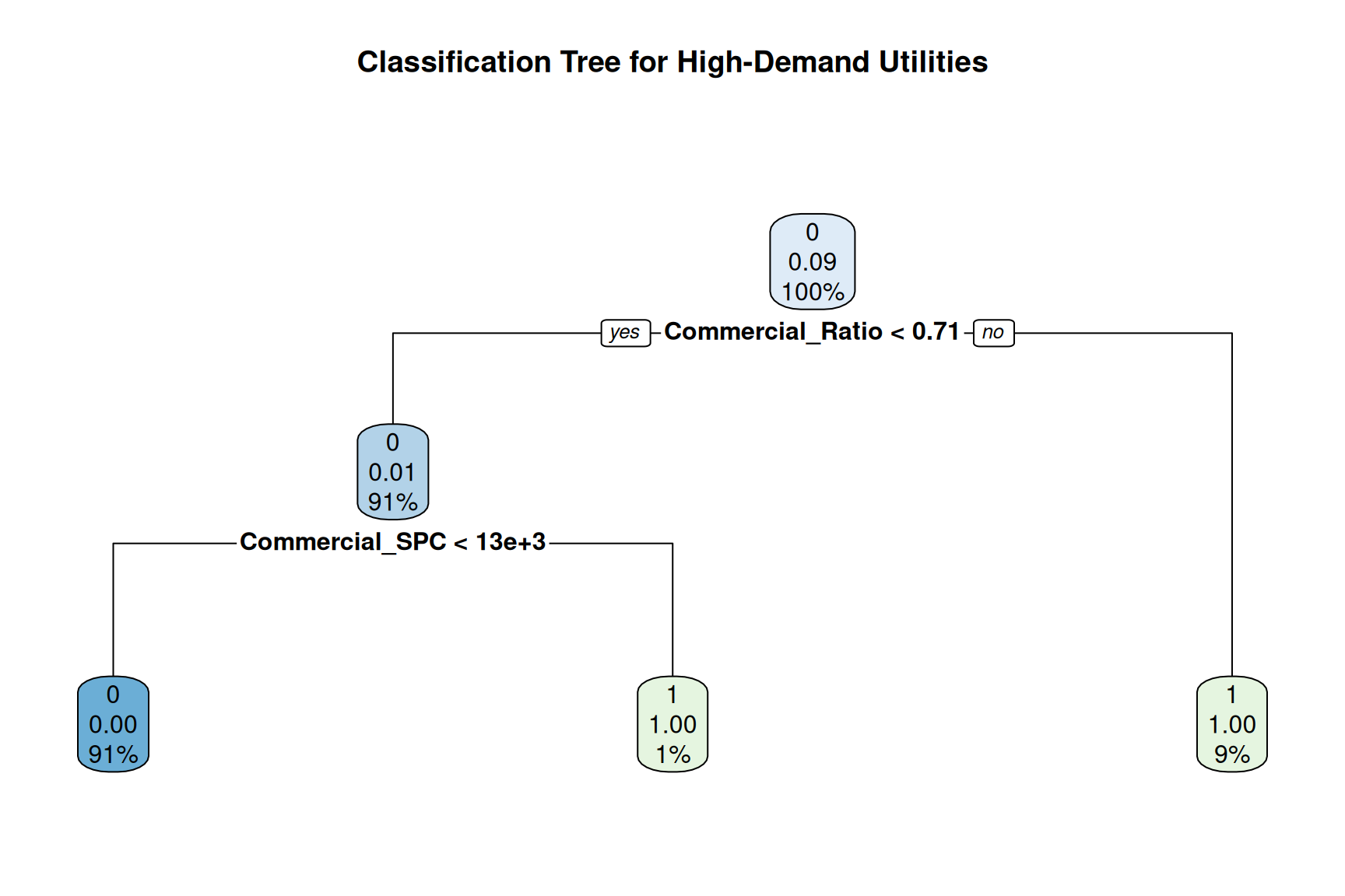

Figure 16: Classification Tree for High Demand Utilities

#Confusion Matrix
confusion_tree <- table(Predicted = tree_pred,
                        Actual    = test$HighDemand_intensity)
kable(
confusion_tree,
caption = "Confusion Matrix (Classification Tree Model)",
align = "c"
)
#Accuracy Table
accuracy_tree <- mean(tree_pred == test$HighDemand_intensity)
kable(
data.frame('Classification Accuracy' = round(accuracy_tree, 4)),
align = "c"
)

Table 5: Confusion Matrix for Tree Model (Test Set)

Confusion Matrix (Classification Tree Model)

	0	1
0	273	1
1	2	38

Classification.Accuracy
0.9904

Random Forest

The following code is used in the Random Forest section.

############################################################
## Random Forest
############################################################

#Random Forest Model
rf_model <- randomForest(
  factor(HighDemand_intensity) ~ Commercial_Ratio + SalesPerCustomer +
    Commercial_SPC + Losses_Ratio + log_Total_Customers +
    is_VA + Utility.Type,
  data = train,
  ntree = 500,
  importance = TRUE
)

print(rf_model)

Call:
 randomForest(formula = factor(HighDemand_intensity) ~ Commercial_Ratio +      SalesPerCustomer + Commercial_SPC + Losses_Ratio + log_Total_Customers +      is_VA + Utility.Type, data = train, ntree = 500, importance = TRUE) 
               Type of random forest: classification
                     Number of trees: 500
No. of variables tried at each split: 2

        OOB estimate of  error rate: 0.4%
Confusion matrix:
     0   1 class.error
0 1132   3 0.002643172
1    2 116 0.016949153

#Variable Importance Visualization
varImpPlot(rf_model, main = "Random Forest Variable Importance")

#Random Forest Predictions
rf_pred <- predict(rf_model, newdata = test)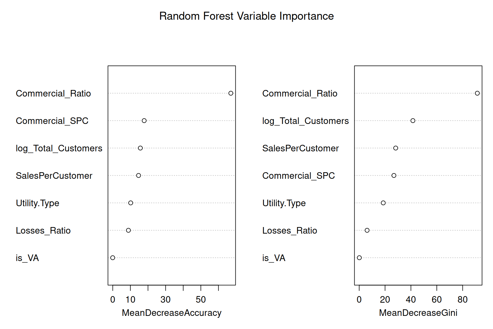

Figure 17: Random Forest Variable Importance

#Confusion Matrix
confusion_rf <- table(Predicted = rf_pred,
                      Actual    = test$HighDemand_intensity)
kable(
  confusion_rf,
  caption = "Confusion Matrix (Random Forest Model)",
  align = "c"
)
#Accuracy Table
accuracy_rf <- mean(rf_pred == test$HighDemand_intensity)
kable(
  data.frame(`Classification Accuracy` = round(accuracy_rf, 4)),
  align = "c"
)

Table 6: Confusion Matrix for Random Forest Model (Test Set)

Confusion Matrix (Random Forest Model)

	0	1
0	273	2
1	2	37

Classification.Accuracy
0.9873

KNN

The following code is used in the KNN section.

# ############################################################
# KNN 
# ############################################################
# 
knn_vars <- c(
  "Commercial_Ratio",
  "SalesPerCustomer",
  "Commercial_SPC",
  "Losses_Ratio",
  "log_Total_Customers"
)

train_means <- sapply(train[, knn_vars], mean, na.rm = TRUE)
train_sds   <- sapply(train[, knn_vars], sd,   na.rm = TRUE)

scale_with_train <- function(df_num) {
  as.data.frame(
    sweep(
      sweep(as.matrix(df_num), 2, train_means, "-"),
      2, train_sds, "/"
    )
  )
}

knn_train_X <- scale_with_train(train[, knn_vars])
knn_test_X  <- scale_with_train(test[, knn_vars])

knn_train_y <- train$HighDemand_intensity
knn_test_y  <- test$HighDemand_intensity

k_val <- 5

knn_pred_test <- class::knn(
  train = knn_train_X,
  test  = knn_test_X,
  cl    = knn_train_y,
  k     = k_val
)

confusion_knn <- table(Predicted = knn_pred_test,
                       Actual    = knn_test_y)
kable(
  confusion_knn,
  caption = "Confusion Matrix (KNN)",
  align = "c"
)
accuracy_knn <- mean(knn_pred_test == knn_test_y)
kable(
  data.frame(`Classification Accuracy` = round(accuracy_knn, 4)),
  align = "c"
)

Table 7: Confusion Matrix for KNN

Confusion Matrix (KNN)

	0	1
0	275	10
1	0	29

Classification.Accuracy
0.9682

PCA and K-means Unsupervised Approach

The following code is used in the PCA and K-means Unsupervised Approach section.

############################################################
## PCA + K-means (Unsupervised)
############################################################

pca_vars <- c(
  "Commercial_Ratio",
  "SalesPerCustomer",
  "Commercial_SPC",
  "Losses_Ratio",
  "log_Total_Customers"
)

X_pca <- df_year %>%
  select(all_of(pca_vars)) %>%
  scale() %>% # z-score standardization
  as.matrix()

pca_res <- prcomp(X_pca, center = FALSE, scale. = FALSE)

# Proportion of variance explained
pca_var <- pca_res$sdev^2
pca_var <- pca_var / sum(pca_var)

scree_df <- data.frame(
  PC = seq_along(pca_var),
  VarExplained = pca_var
)

loadings <- pca_res$rotation  # variable loadings for each PC

label_pc <- function(pc_loadings, pc_name) {
  top_vars <- sort(abs(pc_loadings), decreasing = TRUE)[1:2]
  var_names <- names(top_vars)
  
  sprintf("%s: %s & %s",
          pc_name,
          gsub("_", " ", var_names[1]),
          gsub("_", " ", var_names[2]))
}

pc1_label <- label_pc(loadings[, 1], "Component 1")
pc2_label <- label_pc(loadings[, 2], "Component 2")
pc3_label <- label_pc(loadings[, 3], "Component 3")

# pc1_label
# pc2_label
# pc3_label

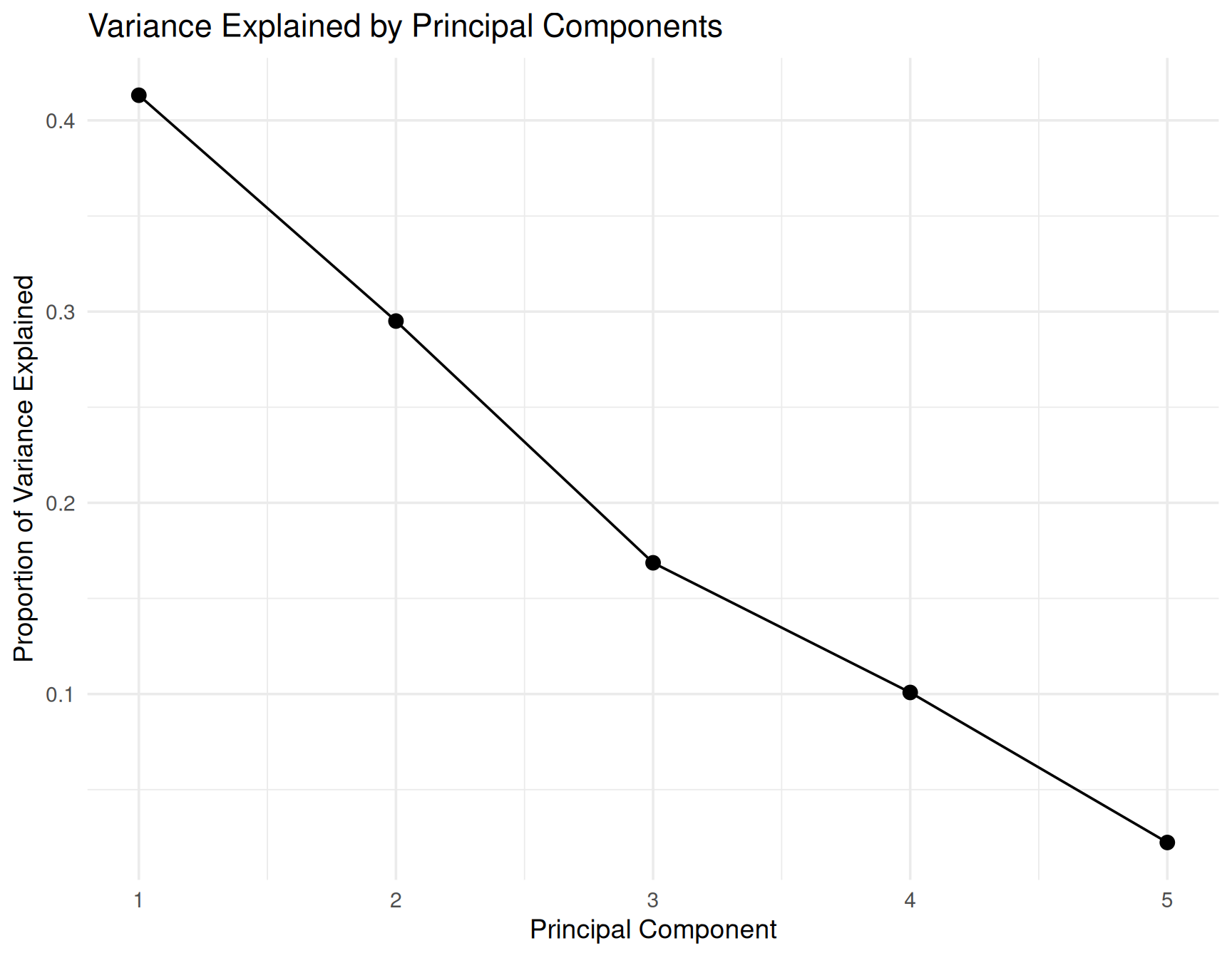
ggplot(scree_df, aes(x = PC, y = VarExplained)) +
  geom_point(size = 3) +
  geom_line() +
  scale_x_continuous(breaks = scree_df$PC) +
  theme_minimal(base_size = 14) +
  labs(
    title = "Variance Explained by Principal Components",
    x = "Principal Component",
    y = "Proportion of Variance Explained"
  )

Table 8: PCA Scree Plot

library(ggrepel)

df_pca <- cbind(df_year, as.data.frame(pca_res$x))

va_utils <- c(
  "Northern Virginia Elec Coop",
  "Virginia Electric & Power Co"
)

annot_df <- df_pca %>%
  filter(Utility.Name %in% va_utils)

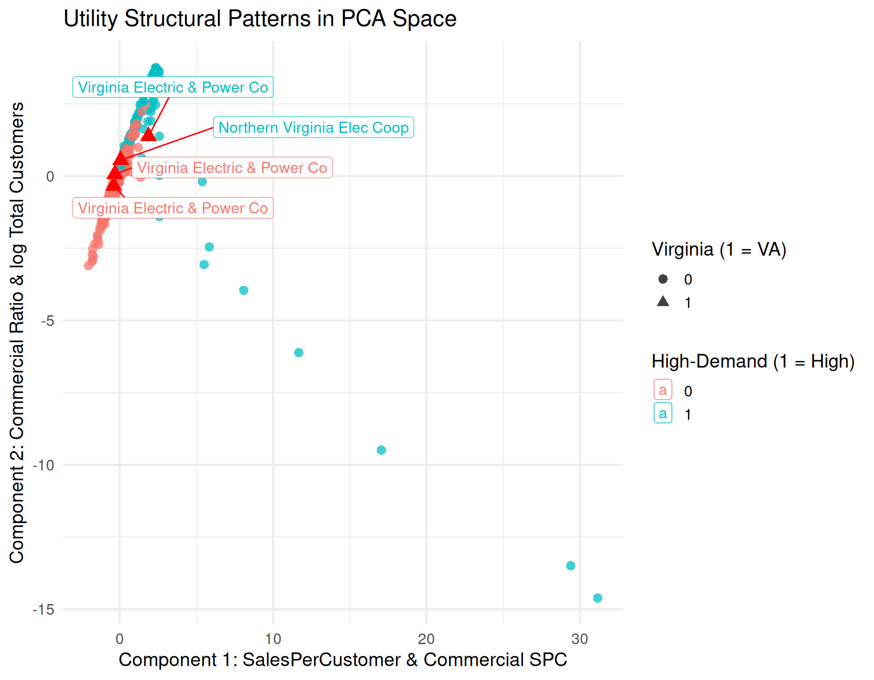
ggplot(df_pca,
       aes(x = PC1, y = PC2,
           color = factor(HighDemand_intensity),
           shape = factor(is_VA))) +
  geom_point(alpha = 0.75, size = 2.8) +
  
  geom_point(
    data = annot_df,
    aes(x = PC1, y = PC2),
    color = "red",
    shape = 17,
    size = 4,
    inherit.aes = FALSE
  ) +
  
  geom_label_repel(
    data = annot_df,
    aes(label = Utility.Name),
    box.padding   = 0.5,
    point.padding = 0.3,
    segment.color = "red",
    size = 4,
    fill = "white",
    label.size = 0.2,
    max.overlaps = Inf
  ) +
  
  theme_minimal(base_size = 14) +
  labs(
    title = "Utility Structural Patterns in PCA Space",
    x = pc1_label,
    y = pc2_label,
    color = "High-Demand (1 = High)",
    shape = "Virginia (1 = VA)"
  )

Table 9: PCA

X_cluster <- df_pca %>%
  dplyr::select(PC1, PC2, PC3) %>%
  as.matrix()

set.seed(123)
k <- 3
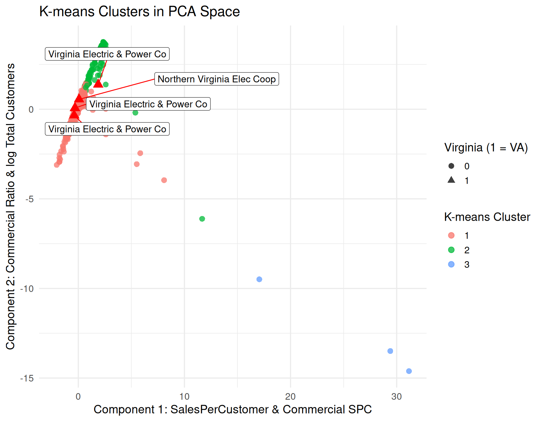
km_res <- kmeans(X_cluster, centers = k, nstart = 25)

df_pca$cluster_km <- factor(km_res$cluster)

ggplot(df_pca,
       aes(x = PC1, y = PC2,
           color = cluster_km,
           shape = factor(is_VA))) +
  geom_point(alpha = 0.75, size = 2.8) +

  geom_point(
    data = annot_df,
    aes(x = PC1, y = PC2),
    inherit.aes = FALSE,
    color = "red",
    shape = 17,
    size = 4
  ) +

  geom_label_repel(
    data = annot_df,
    aes(x = PC1, y = PC2, label = Utility.Name),
    inherit.aes  = FALSE,
    box.padding   = 0.5,
    point.padding = 0.3,
    segment.color = "red",
    size          = 4,
    fill          = "white",
    label.size    = 0.2,
    max.overlaps  = Inf
  ) +

  theme_minimal(base_size = 14) +
  labs(
    title = "K-means Clusters in PCA Space",
    x = pc1_label,
    y = pc2_label,
    color = "K-means Cluster",
    shape = "Virginia (1 = VA)"
  )

Table 10: PCA and K-means Clustering

Model Comparison Summary

The following code is used in the Model Comparison Summary section.

# ############################################################
# Model Comparison Summary (2023)
# ############################################################

model_compare <- data.frame(
  Model = c(
    "Logistic Regression (Raw)",
    "Logistic Regression (Scaled)",
    "Ridge Logistic Regression",
    "Classification Tree",
    "Random Forest",
    "KNN (k = 5)"
  ),
  Accuracy = c(
    round(accuracy_raw, 4),
    round(accuracy_std, 4),
    round(accuracy_ridge, 4),
    round(accuracy_tree, 4),
    round(accuracy_rf, 4),
    round(accuracy_knn, 4)
  ),
  Notes = c(
    "Coefficient explosion; separation issues",
    "Still unstable but standardized",
    "Most stable logistic model; good generalization",
    "Low-variance, simple interpretable model",
    "Highest-performing tree-based model",
    "Sensitive to scaling; depends on local structure"
  )
)

kable(model_compare, align = "c", caption = "Model Performance Comparison") |>
  kable_styling(full_width = FALSE, bootstrap_options = c("striped", "hover", "condensed"))

Table 11: Model Summary

Model Performance Comparison

Model	Accuracy	Notes
Logistic Regression (Raw)	0.9777	Coefficient explosion; separation issues
Logistic Regression (Scaled)	0.9777	Still unstable but standardized
Ridge Logistic Regression	0.9459	Most stable logistic model; good generalization
Classification Tree	0.9904	Low-variance, simple interpretable model
Random Forest	0.9873	Highest-performing tree-based model
KNN (k = 5)	0.9682	Sensitive to scaling; depends on local structure

Results

The following code is used in the Results section.

classify_year_with_models <- function(
  year,
  data_all = power_combined,
  featurizer = featurize_utilities,
  ridge_obj = ridge_cv,
  rf_obj = rf_model,
  formula = formula_all,
  train_data = train,
  x_cols = ridge_x_cols
) {
  df_year_fe <- data_all %>%
    dplyr::filter(Year == year) %>%
    featurizer()

  df_year_fe <- df_year_fe %>%
    dplyr::mutate(
      Utility.Type = factor(
        Utility.Type,
        levels = levels(train_data$Utility.Type)
      )
    )

  if (is.factor(train_data$is_VA)) {
    df_year_fe <- df_year_fe %>%
      dplyr::mutate(is_VA = factor(is_VA, levels = levels(train_data$is_VA)))
  } else if (is.logical(train_data$is_VA)) {
    df_year_fe <- df_year_fe %>%
      dplyr::mutate(is_VA = as.logical(is_VA))
  } else if (is.numeric(train_data$is_VA)) {
    df_year_fe <- df_year_fe %>%
      dplyr::mutate(is_VA = as.numeric(is_VA))
  }

  terms_x <- delete.response(stats::terms(formula))
  X_year <- model.matrix(terms_x, data = df_year_fe)
  X_year <- X_year[, colnames(X_year) != "(Intercept)", drop = FALSE]

  if (!is.null(x_cols)) {
    X_tmp <- matrix(0, nrow = nrow(X_year), ncol = length(x_cols))
    colnames(X_tmp) <- x_cols

    common <- intersect(colnames(X_year), x_cols)
    if (length(common) > 0) {
      X_tmp[, common] <- X_year[, common, drop = FALSE]
    }

    X_year <- X_tmp
  }

  ridge_prob <- predict(
    ridge_obj,
    newx = X_year,
    s = "lambda.min",
    type = "response"
  )
  ridge_class <- ifelse(ridge_prob >= 0.5, 1L, 0L)

  rf_vars <- c(
    "Commercial_Ratio", "SalesPerCustomer", "Commercial_SPC",
    "Losses_Ratio", "log_Total_Customers", "is_VA", "Utility.Type"
  )

  df_for_rf <- df_year_fe %>%
    dplyr::select(dplyr::all_of(rf_vars))

  rf_class <- predict(rf_obj, newdata = df_for_rf, type = "response")

  if (is.factor(rf_class)) {
    rf_class_int <- as.integer(as.character(rf_class))
  } else {
    rf_class_int <- as.integer(rf_class)
  }

  df_year_fe %>%
    dplyr::mutate(
      pred_high_ridge = ridge_class,
      pred_high_rf    = rf_class_int
    )
}

############################################################
## Create classified_all
############################################################

years_to_compare <- c(2018, 2023)

classified_list <- lapply(
  years_to_compare,
  classify_year_with_models,
  train_data = train,
  x_cols = ridge_x_cols
)

names(classified_list) <- years_to_compare

classified_all <- dplyr::bind_rows(
  lapply(names(classified_list), function(yr) {
    classified_list[[yr]] %>%
      dplyr::mutate(Year = as.integer(yr))
  })
)

############################################################
## Proportion of high-demand utilities (Virginia vs national) - Ridge Model
############################################################

state_prop_high <- classified_all %>%
  dplyr::group_by(Year, Utility.State) %>%
  dplyr::summarise(
    n_util = dplyr::n(),
    n_high_ridge = sum(pred_high_ridge == 1L, na.rm = TRUE),
    prop_high_ridge = n_high_ridge / n_util,
    .groups = "drop"
  )

plot_prop_va <- ggplot(
  state_prop_high,
  aes(
    x = reorder(Utility.State, prop_high_ridge),
    y = prop_high_ridge,
    fill = Utility.State == "VA"
  )
) +
  geom_col() +
  coord_flip() +
  facet_wrap(~ Year, scales = "free_y") +
  scale_fill_manual(
    values = c("grey80", "steelblue"),
    labels = c("Other States", "Virginia"),
    name = ""
  ) +
  labs(
    title = "Proportion of Predicted High-Demand Utilities by State (Ridge Model)",
    x = "State",
    y = "Proportion of utilities classified as high-demand"
  ) +
  theme_minimal(base_size = 12)

print(plot_prop_va)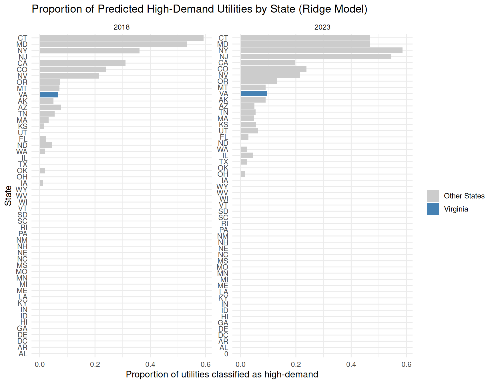

Figure 18: Proportion of high-demand utilities (Virginia vs national) - Ridge Model

############################################################
## Weighted DCLI dominance (retail sales, customers, commercial sales)
############################################################

state_weighted <- classified_all %>%
  dplyr::group_by(Year, Utility.State) %>%
  dplyr::summarise(
    total_retail_sales = sum(Retail.Total.Sales, na.rm = TRUE),
    total_customers = sum(Retail.Total.Customers, na.rm = TRUE),
    total_comm_sales = sum(Retail.Commercial.Sales, na.rm = TRUE),

    high_sales_ridge = sum(dplyr::if_else(pred_high_ridge == 1L,
                                              Retail.Total.Sales, 0),
                               na.rm = TRUE),
    high_customers_ridge = sum(dplyr::if_else(pred_high_ridge == 1L,
                                              Retail.Total.Customers, 0),
                               na.rm = TRUE),
    high_comm_ridge = sum(dplyr::if_else(pred_high_ridge == 1L,
                                              Retail.Commercial.Sales, 0),
                               na.rm = TRUE),
    .groups = "drop"
  ) %>%
  dplyr::mutate(
    prop_sales_high_ridge = dplyr::if_else(
      total_retail_sales > 0,
      high_sales_ridge / total_retail_sales,
      NA_real_
    ),
    prop_customers_high_ridge = dplyr::if_else(
      total_customers > 0,
      high_customers_ridge / total_customers,
      NA_real_
    ),
    prop_comm_high_ridge      = dplyr::if_else(
      total_comm_sales > 0,
      high_comm_ridge / total_comm_sales,
      NA_real_
    ),
    DCLI_ridge = (
      prop_sales_high_ridge +
      prop_customers_high_ridge +
      prop_comm_high_ridge
    ) / 3
  )

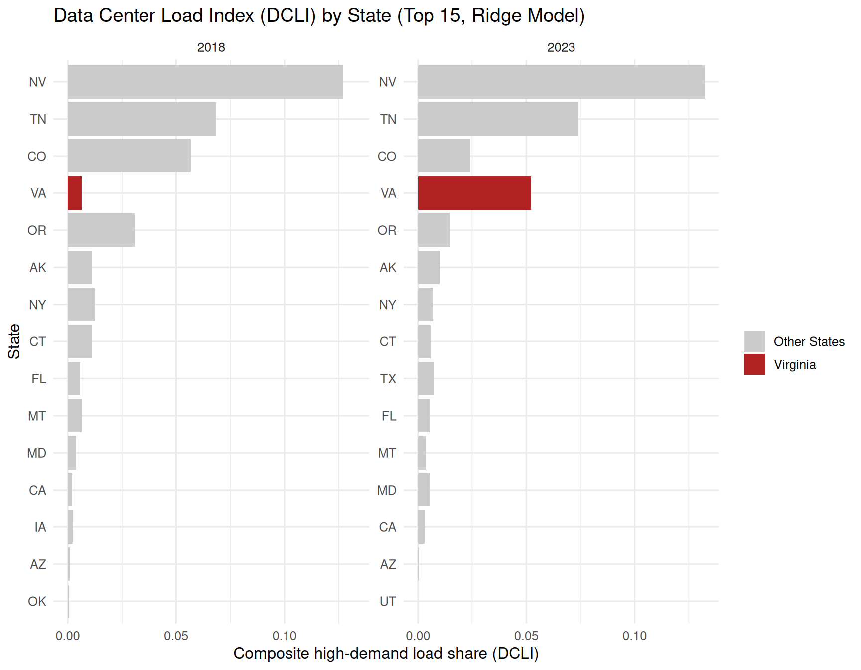
top_states_dcli <- state_weighted %>%
  dplyr::group_by(Year) %>%
  dplyr::arrange(dplyr::desc(DCLI_ridge)) %>%
  dplyr::slice_head(n = 15) %>%
  dplyr::ungroup()

plot_dcli_va <- ggplot(
  top_states_dcli,
  aes(
    x = reorder(Utility.State, DCLI_ridge),
    y = DCLI_ridge,
    fill = Utility.State == "VA"
  )
) +
  geom_col() +
  coord_flip() +
  facet_wrap(~ Year, scales = "free_y") +
  scale_fill_manual(
    values = c("grey80", "firebrick"),
    labels = c("Other States", "Virginia"),
    name   = ""
  ) +
  labs(
    title = "Data Center Load Index (DCLI) by State (Top 15, Ridge Model)",
    x     = "State",
    y     = "Composite high-demand load share (DCLI)"
  ) +
  theme_minimal(base_size = 12)

print(plot_dcli_va)

Figure 19: High-demand utility concentration and weighted dominance across states, highlighting Virginia.